
Loan participations have always followed a cyclical pattern, largely influenced by liquidity. In times of excess liquidity—such as 2020 and 2021—strong demand for loans drove down yields, making trades more competitive. However, the landscape shifted in 2022 and 2023, when tighter liquidity forced sellers to offer deals at historically high spreads to attract buyers.
While liquidity remains a key factor, the introduction of the Current Expected Credit Loss (CECL) model has added a new layer of complexity. Now, buyers are not only evaluating market conditions but also adjusting their strategies based on the CECL reserves required for a given asset class. As the market continues to evolve, understanding these driving forces will be critical for navigating loan participation opportunities effectively.
The CECL model requires financial institutions to estimate expected credit losses over the lifetime of a financial asset at the time of origination. Before CECL, the incurred loss model was used, which only required recognizing credit losses when they became probable. CECL shifts this approach by requiring an estimate of lifetime credit losses from day one based on historical data, current conditions, and reasonable forecasts.
What does this mean for participations? Over the last year, we noticed buyers skew towards loans with a lower CECL reserve, even if the loss-adjusted yield compensates them for the higher expected losses on a given pool. This was not the intention of the CECL reserve implementation. The goal was to simplify how institutions evaluate losses, not push institutions to focus on certain assets over others. Knowing how to properly evaluate the risk-reward trade-off on a given pool can give buyers the confidence to pursue deals others avoid. Analyzing example RV and auto pools side by side illustrates this tension.[1]
| RV | Auto | |
| Balance | $30MM | $30MM |
| Gross Yield | 8% | 6.5% |
| Annual Loss Assumption | 1.25% | .75% |
| WAL | 4 years | 2 years |
| Lifetime Loss Assumptions | 5% | 1.5% |
| Loss-adjusted yield | 6.75% | 5.75% |
| CECL Reserve | $2.03MM | $0.45MM |
| Est. Gross Rev. Over 4 Years | $9.6MM | $7.8MM |
In the above example, for an RV purchase, the buyer would need to set up a CECL reserve of $2.03MM, a number which might spook a potential investor when compared to the $0.45MM reserve for auto. Despite the higher reserve, in this example, the RV pool offers a loss-adjusted return which is 100bps greater than the auto pool. When one considers the difference in the gross yields, a 150bps spread, over the WAL of the RV pool of four years, the $1.8MM earned in excess of the auto yield makes up for the higher CECL reserves.
Given the impact of CECL reserves on a credit union’s financials, it is important to accurately account (and not over account) for the reserves when evaluating a pool. Below we will go over a number of concepts related to losses on participations such as: (i) what parameters drive losses; (ii) how losses on a given pool of loans compare to the losses on the overall seller balance sheet; and (iii) how to use static loss data to establish a baseline for expected losses.
Using static loss data to evaluate expected losses
In static pool analysis, the performance of a cohort of loans is tracked as they age. The cohort will usually be defined as loans that are similar to each other, with that similarity being as granular as is desired by the user. For instance, one can separate auto loans from other loans, or one can go further and separate new autos from used, direct loans from indirect, etc. The loans will also generally be separated by origination date. This allows for comparisons as underwriting policies change over time and it makes the overall analysis simpler.
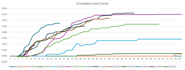
In the loss curve example above, one can see that the cumulative loss curves for recent vintages of sufficient seasoning look to have leveled off around 3.50%. However, the 2022 curve is a bit steeper than the rest. Although it appears to be leveling off near the same level of older vintages, it raises questions:
- Was there a policy change at the credit union?
- A change in servicing practices?
- Is this just an acceleration of the normal amount of losses or will losses rise higher than previous vintages?
It is important to try and answer changes in performance as these need to be incorporated when we estimate losses for a pool’s performance.
Once we have the estimate for cumulative losses, it’s straightforward to convert it into an annual loss estimate by simply dividing the cumulative loss estimate by the WAL.
Anatomy of loan defaults
We analyzed LoanStreet’s database of loans to evaluate what loan parameters drive losses. We strictly focused on auto and our data set included a total original balance equal to approximately $19B across 628k loans.
From this analysis, we determined that LTV and credit scores have the largest impact on expected losses. The biggest jump in losses can be seen when moving to sub 700 credit scores. Elsewhere, migrating from the 760-779 bucket to the 740-759 bucket also results in a relatively large increase in charge-offs. As for LTV, losses picked up significantly above 120%. Loan terms, new/used and direct/indirect also have a significant impact but to a lesser degree.
Understanding what drives losses will help one understand how one pool will compare to another and make the proper CECL reserve adjustments.
Positive selection
When building a pool, LoanStreet applies several filters to a credit union’s loan file, regardless of whether it’s already a subset of loans that the credit union has selected or its entire portfolio. In general, any loan that is more than 20-days past due or has ever been delinquent in the past is excluded. Missing credit scores, DTIs or other critical data points are also excluded. In addition, we will generally filter out credit scores below some threshold (usually 660), DTIs above some threshold (usually 50) and LTVs above some threshold (usually 125). This last step is done primarily to meet as many buyers’ underwriting standards as possible while not being so onerous as to create such a small pool that it doesn’t meet the seller’s objectives.
A side effect of this threshold filtering is it creates a pool that will likely perform materially differently (i.e., better) than the seller’s aggregate statistics might suggest—an important factor to keep in mind when evaluating the pool as a potential purchase.
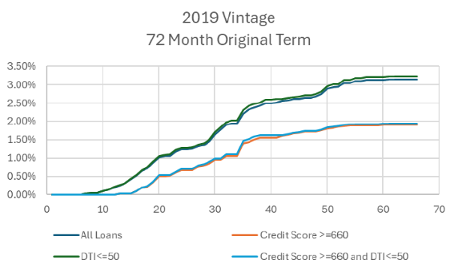
As can be seen, while the DTI filter had little effect, likely due to the limited number of loans excluded, the credit score filter had a material impact, reducing cumulative reported chargeoff amounts from roughly 3.15% to 1.95%, an almost 40% reduction in cumulative losses.
Obviously, the positive selection advantage for every credit union will be different; a credit union that originates nothing but loans that pass the filters would not see any performance improvement while those that originate more loans outside of the filters would see an even greater improvement. It therefore is important to know when evaluating a pool how similar or different it is relative to any performance data one may be utilizing to estimate the credit of the pool and adjust one’s assumptions accordingly.
From a seller’s perspective, the CECL reserve plays an important role as the reserves are released at time of sale. If the reserve set aside was particularly conservative, and the buyer has a more optimistic view of the asset class, a seller would be able to release reserves while selling the loans at a favorable execution.
CECL was meant to provide a single process for how institutions should think about losses and to better prepare them for when losses occur. It was not meant to skew the market to a given asset class based strictly on the amount of reserves required. With the introduction of CECL, however, we have seen many buyers opt for short-term super prime assets, even if it means a lower loss-adjusted return. By knowing how to properly evaluate CECL reserves, buyers are better able to make adjustments to the reserve and gain yield on assets from which other buyers are shying away.
[1] These numbers are strictly for illustrative purposes and are not representative of actual loss assumptions.