
Currently many financial institutions find themselves having excess liquidity and are experiencing net interest margin (NIM) compression.In response, ideas to enhance yield through riskier investments and/or expanding credit boxes to serve lower credit score borrowers are being discussed more frequently.For certain financial institutions, serving lower credit score borrowers is an important part of their core mission.For others, they may have historically lacked the expertise to service those loans well.In either case, it is important to approach this choice in a dispassionate, quantitative manner, that utilizes a consistent risk-pricing framework as used elsewhere in the institution.While extending credit to riskier borrowers on overly generous terms can have negative consequences, it is also rarely the correct decision to declare entire, relatively common, asset classes as off-limits unless the institution simply does not have the framework to understand them.
Defining Your Quantitative Risk Measurement Metric
Every day financial institutions decide whether to place portions of their capital in risk-free assets, such as US Treasuries, or seek higher expected yields in riskier investments or loans.Therefore, whether intentionally or not, these institutions are constantly making judgements that the increased expected after cost yield of these riskier assets adequately compensates them for the increased risk.Moreover, when originating a loan, these institutions furthermore also decide that they have the expertise and operational capacity to service the loan.
While terms such as risk-free yield and expected yield are somewhat intuitive, a Risk Measurement Metric (“RMM”) requires further definition.Although statistical measurements, such as Beta, return variance or standard deviation, are commonly used quantitative RMMs in many areas of asset management, if they are not what an institution already uses, whatever the existing RMM currently in use can still be used absent a determination that it should be changed.However, it is fundamentally important that all institutions have a defined RMM in place.Institutions making loans and undertaking investments without any explicit method of measuring relative risks need to “discover” the quantitative RMM already being implicitly used to guide their decisions for evaluating future opportunities.
How to Quantitatively Compare Opportunities
To compare opportunities with different expected yields, servicing costs, and risk profiles it is necessary to introduce additional mathematical rigor, even if we don’t explicitly define the RMM to be used or address the merits of different RMMs that could be used:
Rf = risk-free yield
SC = servicing cost for the originating institution (or the assessed one by the servicer)
R(e)1 = expected yield on asset 1
RMM1 = Risk Measurement Metric for asset 1
A principle starting point is that risky assets should offer a higher expected return than risk-free assets.When originating a non-risk-free loan or purchasing a participation in a non-risk-free loan this can be expressed as follows:
R(e)1 – SC > Rf
The next step is then to address how much higher does the after cost expected yield need to be than the yield on a comparable risk-free asset.Fundamentally, for any asset purchased or loan originated, institutions must estimate both expected after cost return and the corresponding RMM.This allows the net expected yield in excess of the risk-free rate on different assets to be reasonably and methodically compared.For example, let’s say we want to assess whether new-Asset 2 is offering a sufficiently high expected yield versus less-risky Asset 1 where capital is already routinely deployed:
Asset 1 Reward For Risk Ratio (“ARRR1”): (R(e)1 – SC1 – Rf) / RMM1
Asset 2 Reward For Risk Ratio (“ARRR2”): (R(e)2 – SC2 – Rf) / RMM2
If ARRR2 is greater than ARRR1, then Asset 2 offers a superior risk-return profile to Asset 1.If “return standard deviation” is the institution’s chosen RMM, these ratios are the familiar Sharpe ratios most commonly employed in equities analysis and we would equivalently conclude that Asset 2 has a higher/better Sharpe ratio than Asset 1.
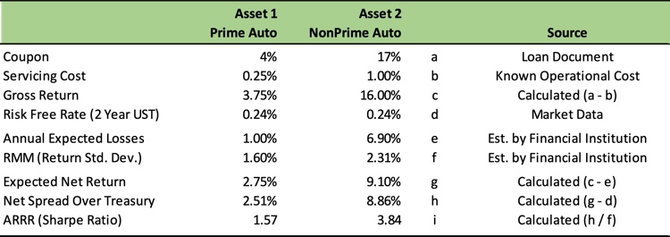
Let’s look at an example calculation of the ARRR, and also in this case a Sharpe ratio, for two auto loan pools.In this example the nonprime auto pool offers superior return for risk versus the prime auto pool and we reach that conclusion because its ARRR (Sharpe ratio) is higher.Notably, the only estimated inputs are the annual expected losses and the RMM, here defined as the return standard deviation which would most typically be calculated by reviewing the historical return volatility of similar assets.All other figures are known inputs from easily accessible sources.
Beyond ranking the desirability of specific assets at a point in time, institutions can also adopt a more generalized screening approach for evaluating whether opportunities meet risk-return requirements by setting a required Minimum Reward for Risk Ratio (“MRRR”), below which opportunities will be ruled-out in favor of non-risk-free opportunities that exceed the MRRR or Treasuries.
Required Minimum Reward for Risk Ratio (“MRRR”)
(R(e) – SC – Rf) / RMM > MRRR
Revisiting Entering Nonprime
By utilizing a quantitative approach to evaluate all non-risk-free opportunities we can return to the original question of whether it makes sense for an institution to expand into nonprime loans.Specifically, if ARRRnonprime > ARRRprime then the nonprime opportunity offers a superior reward for the amount of risk.That said, there is considerable expertise involved in estimating ARRR and it important any institution entering the nonprime space can assess (or rely upon others to assess) the following:
- Can my organization make an informed view of the expected return?
- Can my organization reliably estimate the risk of this asset (on a similar apples-to-apples RMM as already done for existing assets on the balance sheet)?
- For buying participations: do we assess the underwriting practices of the originator and the capabilities of the servicer favorably?
- For originating: does our organization have the resources to efficiently execute servicing?
Institutions that can not make reasonably informed expected return nor risk estimates on nonprime loans should avoid the asset class.However, many institutions that do not presently originate nonprime loans can assess these assets quite well and may be needlessly constraining themselves, and suffering more severe NIM compression, due to seemingly prudent investment policies that limit nonprime exposure.Purchasing participations in nonprime loans could be an emerging vehicle for these institutions to benefit from higher risk-adjusted expected returns without needing to make large operational investments in nonprime origination and servicing capabilities.
Co-authored by Michael Lanzarone