Not from concentrate: Portfolio diversification with loan participations

While many loan sales are made up of new loans, some sales consist of seasoned loans that are several or more years old. Because the likelihood of prepayments and defaults changes as loans mature, evaluating pools requires accounting for the effects of this aging. The effects of seasoning on expected prepayments and defaults rates can not only be material, but also make seasoned pools compelling purchase opportunities.

To explore these opportunities, one should create a loss-timing curve to investigate the likelihood of default over time. In general, prepay and default rates rise during the infancy of a loan’s life, reach a peak or plateau, and then decline. Prepayment curves usually have similar shapes to loss-timing curves like this one (though prepayments for a post-peak seasoned pool will usually not decline as much as losses, and will sometimes rise towards the end of the loan):

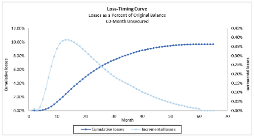
For prepayments, it is unlikely for someone who just received a loan to entertain applying for a new loan to pay off an existing one. Towards the end of the life of the loan, prepayments will often rise as the borrower looks to pay it off in full. For defaults, it’s generally less likely that a newly-underwritten loan will fail as financials and due diligence are verified. On the other hand, as a loan nears maturity, defaults decline because the remaining payments are unlikely to burden the borrower. However, in between those stages, there are many reasons why borrowers are no longer willing or able to repay the loan.

Incorporating projected balances into the equation

When using loss curves to analyze the purchase of seasoned loans, one needs to think in terms of annual losses. To do this, consider what has been happening to the pool balance as it declines through amortization and paydowns. By taking the remaining cumulative losses at any given time and dividing it by the pool balance at that same time, we can estimate losses as a percentage of the outstanding pool balance. If this estimate is then divided by the weighted-average life or modified duration of the loan, we can calculate an expected annual loss rate.

For instance, using the example from above and assuming a Conditional Prepayment Rate (CPR) of 30%,  the following curve represents the projected losses as a percentage of the remaining balance (assuming past due loans are excluded from the pool at each point of seasoning):

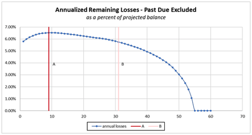
If a buyer purchases this loan pool on or after Point B, AFTER the majority of the losses have taken place, they will experience lower annualized losses than at any earlier time. However, if the buyer purchases this loan pool at Point A, AFTER the initial period when defaults are less likely but BEFORE the steep part of the curve begins, they should expect higher annual losses relative to having purchased at origination. This buyer is still expecting the majority of the losses for the pool but has experienced some amount of amortization and prepayments and will have purchased a lower outstanding balance.

Seasoned loan pool analysis in practice

The goal is to arrive at an expected annual loss rate which you can then compare to other expected annual loss rates. The first step is to create loss-timing curves for any assets being evaluated. This can be performed in advance and should represent the percentage of cumulative losses that will occur up to any point of seasoning, ending at 100%. There are numerous sources for this data – a buyer’s historic performance, loan originators’ due diligence loss reports and rating agency data, among others. In cases where the pool is cleaned out of past-due loans, an adjustment needs to reflect this; excluding losses that occur over the next several months can capture this effect. Once these curves are created, they can be referenced in future analyses of new or seasoned pools.

To calculate the expected annual loss rate:

1. Estimate the pool factor based on a prepayment assumption layered on top of the expected amortization of the pool.
2. Divide the remaining loss figure by the pool factor to determine the loss factor.
3. Estimate the expected cumulative losses for the pool being analyzed, as if the loans were new.
4. Multiply the expected cumulative losses by the loss factor to determine the losses as a percent of the current pool.
5. To determine the expected annual loss rate, divide the losses as a percent of the current pool by the weighted-average life or modified duration of the pool.
6. The annual loss rate is then used to estimate the loss-adjusted yield by subtracting it from the non-loss-adjusted yield.

This calculation can be used repeatedly on similar assets, and loss factors can be set up in a spreadsheet and referenced as new pools are evaluated. Just use the appropriate loss factor, estimate the new pool’s expected cumulative losses, multiply the two, and then divide by the weighted-average life or modified duration. The result is the expected annual loss rate.

Conclusion

The key to evaluating seasoned loan pools is recognizing the pattern that the annual loss expectations follow. These expectations rise slightly for the first few months of a pool’s life, then level off, and finally decline as a pool reaches maturity. The shape of these expectations is the result of the interaction between the loss-timing curve and the pool factor. For decision makers overseeing loan portfolios, significantly seasoned pools can present compelling purchase opportunities if they can be shown to project materially lower annualized loss rates than newer pools.

Co-Author: Mark Rambler